Computationally expensive matrix inversion

Hi all,

Last week I wrote a small MATLAB code to compute the result of some theoretical calculations I made.
These calculations are aimed to extract the spectral function A(\mathbf{k},\omega) from the Green’s function (\mathcal{G}) derived using Dyson’s equation and the self-energy (\Sigma).
The purpose of the code Is to compute the self energy (product of know matrices), then the Green’s function and finally extract the spectral density:

[\mathcal{G}_0(\omega)]_{\mathbf{k}, \mathbf{k}'}= \frac{\delta_{\mathbf{k}, \mathbf{k}'}}{\omega-\epsilon_{\mathbf{k}}+i0^+}\\ \mathcal{G}= \big[\mathcal{G}_0^{-1}-\Sigma\big]^{-1}\\ A(\mathbf{k},\omega)= -\frac{1}{\pi} \Im\big([\mathcal{G}(\omega)]_{\mathbf{k,k}}\big)

with \epsilon_\mathbf{k} single-particle unperturbed energy and \mathcal{G}_0 non-interacting Green’s Function.
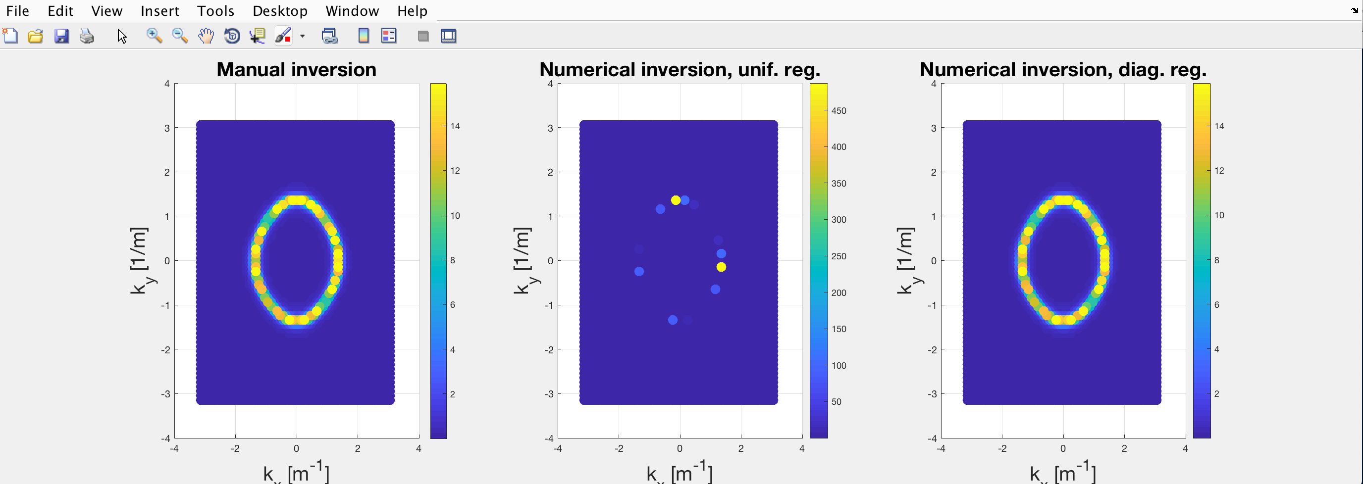
When it came to testing the code, I set the interaction potential to be zero, so that \mathcal{G}\rightarrow \mathcal{G}_0. However, the result was something like this:

Schermata 2020-08-21 alle 23.16.11

where the colorbar is proportional to A(\mathbf{k}, \omega).

The leftmost plot is derived from the “manual” inversion of \mathcal{G}_0 (replaced the each diagonal element with its inverse) and represents the normal parabolic dispersion of the noninteracting modes. On the other hand, the central and rightmost plots are both derived from the numerical inversion of (\mathcal{G}_{0}^{-1}-\Sigma) which is diagonal as \Sigma=0. Since the interaction is null, the three plots should be identical.

I tracked down this issue to the matrix inversion function required to compute \mathcal{G} .
I understand this being a consequence of the size of the matrix (thousands by thousands of elements) which causes the determinant to easily exceed what can be stored in a double.I tried several different functions pinv(), \ and inv() which gave all the same unsatisfactory result.

Therefore my questions are:

  1. Could there be some benefit by moving the code to a different language (Python, C)?
  2. Could it be beneficial to use an external computational cluster to solve the issue?
  3. Is there a more clever way of addressing the problem instead of inverting a huge matrix?

Apologies for the lengthy question but I felt that it needed some context.

2020-08-21T22:00:00Z

1 Like

Great question with a lot of aspects to unwind. It’s also not immediately clear what exactly you are doing, do you mind sharing the minimal code to reproduce the problem?

Here’s a minimal code in Python that demonstrates that matrix inversion itself is not to blame.

import numpy as np
rng = np.random.default_rng()
size = 1000
data = np.exp(10 * rng.normal(scale=10, size=size)) * (2 * rng.integers(0, 2, size) - 1) + 0.j
matrix = np.diag(data)
print(f'condition number = {np.linalg.cond(matrix)}')
print(f'error = {np.linalg.norm(np.diag(np.linalg.inv(matrix)) - 1/data)}')

It prints

condition number = 7.357532487589488e+269
error = 0.0

Here I create a very poorly conditioned diagonal matrix, invert it, and compare the diagonal with the inversion of the original values. I’d be losing up to 269 digits of precision (out of 16 digits that a floating point number accommodates), but since the matrix is diagonal there’s still no error.

While my demonstration is in Python, the linear algebra routines used by essentially all programming languages are actually the same, and I expect an analogous MATLAB code would have the same output.

Thank you for your quick answer Anton.

Here is the minimal code:

%% Minimal code
beta=0.1;
[kx, ky]= meshgrid([-pi:0.1:pi],[-pi:0.1:pi]);       % define k-space
omega=0.5;                                           % choose target frequency

% define dispersion relation
KX=kx( :);
KY=ky( :);
epsilon_k= (1+beta-0.5*cos(KX)-0.5*cos(KY));

% define small regularization
reg=0.02*1i;
regularization_u= ones(numel(KX))*reg;                 %uniform
regularization_d= diag(ones(numel(KX),1)*reg);         %diagonal

%calculate free Green's function

G0m=diag((omega-epsilon_k+reg).^(-1));                          % "manual inversion"
G0n_u= inv(diag(omega-epsilon_k)+regularization_u);             %numerical inversion;
G0n_d= inv(diag(omega-epsilon_k)+regularization_d);             %numerical inversion;

%extract corresponding spectral functions:
Akomega_m=-1/pi*imag(diag(G0m));
Akomega_n_u=-1/pi*imag(diag(G0n_u));
Akomega_n_d=-1/pi*imag(diag(G0n_d));

%%  then plot:
figure(); 
subplot(1,3,1); 
s=scatter3(KX, KY,Akomega_m, 100, Akomega_m, 'filled'); 
subplot(1,3,2); 
s=scatter3(KX, KY,Akomega_n_u, 100, Akomega_n_u, 'filled');
subplot(1,3,3); 
s=scatter3(KX, KY,Akomega_n_d, 100, Akomega_n_d, 'filled');

While writing the minimal code I found the cause of the bug. It looks like it is rather a consequence of the way I introduce the regularization. If the regularization is introduced only on the diagonal, the result from the manually and numerically inverted matrices coincide. On the other hand, when the regularization is added to all the elements of the matrix, the error occurs.

Schermata 2020-08-24 alle 11.47.12

This is compatible with what you have shown in your example, as I see that you added a regularization (0.j) only on the diagonal as well.
As for the central plot, the condition number is cond(G0_n)= 3.6e+06. I don’t know if this is enough to blame numerical errors for the discrepancy…
Do you think that this could be the cause? If yes, is there a workaround for this issue? because I will still need to invert matrices which are not diagonal and may be ill conditioned.

Adding 0j only converts an array to complex, it’s not actually a regularization. Adding a constant quantity to each element is indeed an incorrect way to regularize the matrix.

That still leaves you with 10 digits of precision even before you add Σ (which would typically make everything better behaved).

Thank you very much Anton :slight_smile:

Have a good day.

1 Like